Topology and Geometry in Physics

Homeomorphism is a continuous map from one topological space to another, with a continuous inverse. That is, two spaces are homeomorphic if they can be transformed continuously to one another without cutting or pasting. Homeomorphic spaces are topologically equivalent. Some of the topological invariants include connectedness, compactness and Euler characteristic which for a polygon is the (number of vertices) - (number of edges) + (number of faces).

Sphere The sphere $S^2$ is not homeomorphic to any open subset of ${ℝ}^2$ as the former is compact i.e. closed and bounded, while the latter is not. However, a sphere with a hole is homeomorphic to a disc $D^2$.

By $C_r(K)$, let us denote the free abelian group of all r-dimentional oriented volume elements of a topological space K such that $c={\sum }_i{c}_i{\sigma }_i\in C_r(K)$ if ${\sigma }_i\in C_r(K)$, $c_i\in \mathbb{Z}$. For $r=1$ it can be all curves, for $r=2$ it can be all surfaces, and so on.
By $Z_r(K)$, we mean group of all elements of $C_r(K)$ that are r-cycles i.e. they do not have a boundary, which can happen if the boundary elements add up to 0. For example, closed loops. For a triangle the boundary is given by

where $p_i$ is a point and $(p_i{p}_j)$ is an oriented line segment.
By $B_r(K)$ we mean group of all elements of $C_r(K)$ that are boundaries of $C_{r+1}(K)$. It can be shown that $B_r(K)\subseteq Z_r(K)$.
Then the homology group is $H_r(K)\equiv Z_r(K)/B_r(K)$, which is the group of r-cycles which are not themselves the boundaries of some element in $C_{r+1}$.

Circle Let $K=S^1$ i.e. a circle. $Z_1(K)$ is the free group generated by the closed loops which in this case only consist of the circle. Hence $Z_1(K)\cong \mathbb{Z}$. However, $C_2(K)$ is empty and hence so is $B_1(K)$. Therefore,

One isomorphism map from $H_1$ to $\mathbb{Z}$ can be the winding number.

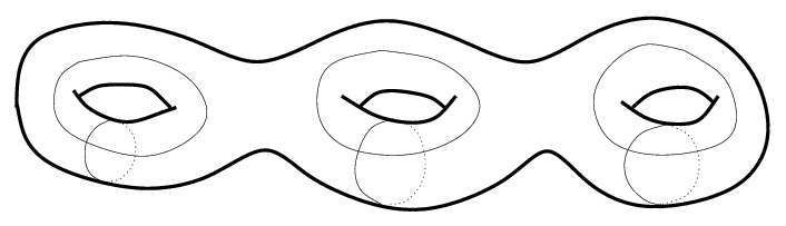
General surface Let K be the most general orientable two-dimensional surface consisting of a 2-sphere with h handles and q holes.
Each handle can be thought of as a torus $(T^2)$ attached to the rest of the object. The first homology group of the torus is generated by two cycles i.e $H_1(T^2)\cong \mathbb{Z}\oplus \mathbb{Z}$. Each hole adds one cycle to the first homology group, which can be seen by taking a loop around the hole. However, adding one loop from around each hole gives a contractible loop and is $\sim$ 0. Therefore,

Two loops in a topological space are said to be homotopic if one can be continuously deformed into another. The product of two loops having a common point is the loop defined as: start from the common point, go around the first loop once and then the second loop once, reaching back to the starting point. Homotopy is an equivalence relation and the equivalence classes of loops hence formed in the topological space is the fundamental homotopy group of the space, denoted by ${\pi }_1(K)$. If the elements of this group commute, this group is isomorphic to the first homology group $H_1(K)$.

It is not always possible to define a coordinate system on a topological space such that it is continuous everywhere and all close points have nearby coordinates. In such cases we use multiple coordinate charts, each defines coordinates locally on open subsets of space such that at points where more than one charts are defined, map from one to another should be smooth. A topological space together with set of charts covering the space, collectively called an atlas, is a manifold.

For example, if we use polar coordinates for sphere, we have a discontinuity as the point $(0,\pi /2)$ is very close to the point $(2\pi -ϵ,\pi /2)$ for small $ϵ$, whereas, the coordinates are far. If we use stereographic coordinates from north pole, we get arbitrarily large coordinates for points close to north pole, they do not have close coordinate representations. Charts are homeomorphisms from open subsets of M to open subsets of ${ℝ}^m$, and being able to represent the sphere with a single chart would mean that sphere is homeomorphic to an open subset of ${ℝ}^2$, which is not true. Hence we need atleast two charts to cover a sphere. We will see an example of sphere manifold wen we study Dirac monopoles.

A smooth curve in a space M is a smooth map $c:ℝ\to M$. Given a curve c and a function $f:M\to ℝ$, we can compose them and then differentiate to get

where $x^{\mu }(p)$ gives the coordinate of point p in M and $X^{\mu }\equiv d{x}^{\mu }(c(t))/dt$. The map

is a tangent vector at p with $\partial /\partial x^{\mu }$ as the coordinate basis. The space of tangent vectors at point p is the tangent space $T_{p}M$. Under change of coordinate system, the components will transform as

This transformation defines a contravariant vector.

The differential 1-form of a function, $f:M\to ℝ$, is a dual to the tangent vector defined by

The space dual to tangent space $T_{p}M$ is the cotangent space $T_p^{\ast }M$. $d{x}^{\mu }$ gives a basis for $T_p^{\ast }M$ dual to the coordinate basis of vector

Under change of coordinate system, the components of the dual vector ${\omega }_{\mu }d{x}^{\mu }$ transform as a covariant vector

A map $f:M\to N$ between two spaces induces a map $f_{\ast }$ called the differential map $f_{\ast }:T_{p}M\to T_{f(p)}M$, such that

Another induced map is the pullback map $f^{\ast }:T_{f(p)}^{\ast }N\to T_p^{\ast }M$ defined by

Mechanics In a configuration space Q, where $q^i$ are local coordinates and $v^i=f{q}^i/dt={\dot{q}}^i$ is the velocity of the dynamical trajectory q(t), a Lagrangian $L(q^i,v^j)$ is a function on the tangent bundle $L:TQ\to ℝ$. The tangent bundle is mapped to its cotangent bundle $T^{\ast }Q$ by the Legendre transformation via

The fact that the momentum lies in the cotangent space can be seen from its covariant transformation under change of coordinate basis. If the above map is invertible, which can happen if the Lagrangian is a convex function of the $v^i$, we obtain an isomorphism between tangent and cotangent bundle, which is very similar to the Wave-Particle Duality where the particle velocity can be obtained from the wave vector. The Legendre transform of the Lagrangian with respect to fibre coordinates is the Hamiltonian

Since, H and L are invariant under coordinate basis change, we see another reason why momentum should be dual to the position.

A tensor of type (q,r) is a multi-linear map $:{⨂}^q{T}_p^{\ast }M{⨂}^r{T}_{p}M\to ℝ$, written in terms of the basis as

A tensor of type (0,r) is a covariant tensor of rank r. A continuous assignment of an element of ${\mathrm{\Im }}_{r,p}^{q}M$ at each point $p\in M$ is a tensor field, where ${\mathrm{\Im }}_{r,p}^{q}M$ is the set of type (q,r) tensors at point p. If $(q,r)=(0,1)$ it is a co-vector field, and if (1,0) it is a vector field.

A differential q-form is an antisymmetric tensor of type (0,q). The vector space of q-forms acting on ${⨂}^p{T}_{p}M$ is denoted by ${\mathrm{\Lambda }}^q(T_{p}M)$. Dim ${\mathrm{\Lambda }}^q(T_{p}M)=\left(\genfrac{}{}{0pt}{}{n}{q}\right)$, where n is the dimensions of $T_{p}M$. ${\mathrm{\Lambda }}^0(T_{p}M)=ℝ$ by convention.

The exterior product is an antisymmetric tensor product $\wedge :{\mathrm{\Lambda }}^q(T_{p}M)\times {\mathrm{\Lambda }}^r(T_{p}M)\to {\mathrm{\Lambda }}^{q+r}(T_{p}M)$ such that

where $V_i\in T_{p}M$. The exterior product of r one-forms is

For example, $d{x}^{\mu }\wedge d{x}^{\nu }=d{x}^{\mu }\otimes d{x}^{\nu }-d{x}^{\nu }\otimes d{x}^{\mu }$.

The direst sum of vector spaces ${\mathrm{\Lambda }}^q(T_{p}M)$, ${⨁}_{q=0}^n{\mathrm{\Lambda }}^q(T_{p}M)$, is denoted by ${\mathrm{\Lambda }}^{\ast }(T_{p}M)$, and along with the exterior product forms an algebra.

The exterior derivative d is a map ${\mathrm{\Lambda }}^r(T_{p}M)\to {\mathrm{\Lambda }}^{r+1}(T_{p}M)$ whose action on an r-form

where ${\omega }_{{\mu }_1\mathrm{\dots }{\mu }_r}$ is totally antisymmetric, is given by

The action of $d^2$ on $\omega$ is

as ${\partial }^2{\omega }_{{\mu }_1\mathrm{\dots }{\mu }_r}/\partial x^{\lambda }\partial x^{\nu }$ is symmetric with respect to $\lambda$ and $\nu$ while $d{x}^{\lambda }\wedge d{x}^{\nu }$ is antisymmetric.

Electromagnetic potential $A=(\varphi ,𝐀)$ is a one-form, $A=A_{\mu }d{x}^{\mu }$. The Electromagnetic tensor F is defined by $F=dA$.

where

Using the identity $d^2=0$ we get two of the Maxwell’s Equations,

From the identity $d^2\omega =0$, we see that the potential $\tilde{A}=A+d\mathrm{\Lambda }$ leads to the same electromagnetic tensor as A. Hence, we expect the trajectory of the particle to remain same under such gauge transformation. For the time-independent electromagnetic fields, $d\mathrm{\Lambda }$ can be replaced by $\nabla \mathrm{\Lambda }$.

The Hamiltonian for the system is given by

and the kinematical momentum is given by

Therefore, if the states change as $|\psi ⟩\to |\tilde{\psi }⟩$ under gauge transformation, we expect

These conditions are satisfied by the transformation

validity of which can be verified by comparing the original with the transformed Schrodinger equation.

Although magnetic monopoles have not yet been found and Quantum Mechanics does not predict their existence, Dirac observed that if monopoles were to exist, it would lead to quantization of magnetic and electric charges.

Consider time-independent electromagnetic fields. In this case, the curvature tensor equals the magnetic field i.e.

Dirac monopole introduces a singularity and hence, to describe it we use two coordinate patches $U_{\pm }$ to describe the $z>-ϵ$ and regions of ${ℝ}^3-\{0\}$ with overlap region $U_{+}\cap U_{-}$ effectively equal to the x-y plane with z=0 minus the origin. We define the vector potentials in the two regions as

The two potentials are related by the gauge transformation

and hence give the same field. $A_{+}$ and $A_{-}$ have the Dirac string singularities at $\theta =\pi$ and $\theta =0$ respectively, however these strings lie outside the coordinate patches their respective potentials are defined in, and we get a genuine singularity only at $r=0$.

Accordingly the gauge is given by

which we see is singular at $\theta =0,2\pi$. But we use the transformation only at $\theta =\pi$ and hence the singularities do not show up in analysis.

The curvature of A is given by

Hence the magnetic field is given by

and the flux is

In analogy with electric charge, g can be identified as a measure of magnetic charge.

For this gauge, the wave-functions transform as

We require the wave-function to be single valued as we go from $\varphi =0$ to $\varphi =2\pi$ along the equatior, which gives us the Dirac quantization condition

We see that at the equator, the transition function is of the form $e^{\iota n\varphi }$, and hence maps the equator $S^1$ to U(1), the integer n characterizing the fundamental homotopy group ${\pi }_1(U(1))=\mathbb{Z}$.

An interesting point in this analysis is that the quantization is not due to the discreteness of the spectrum of an operator in Hilbert space but rather due to topological considerations.

The molecules of nematic liquid crystals are like rods with heads and tails. But they possess inversion symmetry and hence the orientation of a molecule can be described by a point on a sphere with antipodal points identified, i.e the real projective space $ℝP^2$. The map $n(𝕣):{ℝ}^3\to ℝP^2$, which describes the configuration at each point in the crystal space is called the texture.

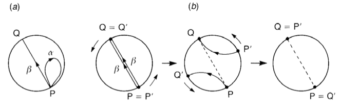
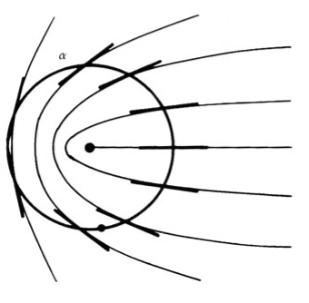
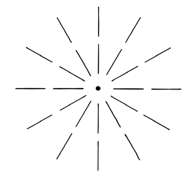
Line Defects We see from the figure that ${\pi }_1(ℝP^2)\cong {\mathbb{Z}}_2=\{0,1\}$. Therefore, there are two kinds of line defects in nematic liquid crystals, one can be continuously transformed into uniform configuration while the other cannot. More specifically, we take a loop $\gamma$ around a line separated from the singular region by few molecular lengths so that the texture is well defined along the loop. The function $n(𝕣)$ maps $\gamma$ to some closed contour $\tau$ in $ℝP^2$. $\tau$ may be of two types: (i) it starts and ends at the same point (for example, a circle) or, (ii) it connects the diametrically opposite points of $S^2$ which are equivalent in $ℝP^2=S^2/Z_2$. Contours of type (i) can be shrunk to a point, while contours of type (ii) cannot be, as shown in the part (a) of above figure. The latter represent stable vortices. They result from spontaneous symmetry breakdown and represent deviations from minimum energy configurations, contributing significantly to the gradient energy which makes their transformation into uniform configuration energetically almost impossible. In nematic liquid crystals it requires destruction of the nematic order in the whole half plane ending at the line. Two vortices of same type may however be deformed into one another with some expenditure of energy.

Bibliography

- [1] Nakahara M. (2003). Geometry, Topology and Physics. Ed. Brewer D.F. 2nd ed. IOP Publishing
- [2] Poletti S.J. (1995). Topological Defects. Lecture Notes, University of Adelaide
- [3] Dirac P.A.M. (1931). Quantised Singularities in the Electromagnetic Field. Proc. R. Soc. Lond. A 133, 60-72
-
[4]
Nash C. (1997). Topology and Physics - a historical essay.
arXiv:hep-th/9709135v4 - [5] Sakurai J.J. (2011). Modern Quantum Mechanics. Ed. Tuan S.F. Revised ed. Pearson
- [6] Eguchi T., Gilkey P.B., Hanson A.J. (1980). Gravitation, Gauge Theories and Differential Geometry. Physics Reports 66, No. 6, 213-393
- [7] Lavrentovich O.D. (2001). Nematic Liquid Crystals: Defects. Encyclopedia of Materials: Science and Technology, 6071-6076. Elsevier Science
[8]
Gibbons G.W. (2006) Applications of Differential Geometry to Physics.
Part III Lecture Notes, DAMTP, Cambridge University